
Looking past the transitory with a focus on secular trends
Concerns over inflation continue to dominate the marketplace. June’s 0.9% rise in core CPI was well above forecasts, as were the April and May prints. Bond yields (which are used to discount risk assets) have oscillated between a high of 1.77% in March to 1.3% recently, as concerns over inflation (and new corona virus variants) have waxed and waned. This in turn has influenced the tug of war between the performance of safety/defensive assets and cyclical reflation assets. Thus far, market consensus data indicate a belief that the sharp price increases have largely been transitory. While we are sympathetic to this view, we also recognize that there is a psychological element to inflation which could be triggered if current conditions are sustained. More importantly, there are larger secular trends that could lead to a regime change from one of low/stable inflation to higher and more volatile inflation levels. For investors, such an environmental shift could both change the performance of different asset classes and upend the fundamental premise underpinning investors’ asset allocation models; that stocks and bonds are likely to be negatively correlated and naturally diversifying. In the second of our 2019 three-part series on portfolio risk strategies, we examined these changing relations in periods of high inflation and stagflation. We conclude this research note with an update of that analysis.
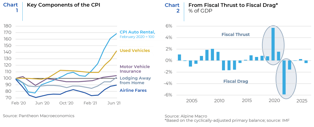
This year’s inflation jumps were largely caused by a combination of base effects, a spike in the prices of products that are in high demand as the world exits pandemic-lockdown restrictions, supply chain disruptions, and monetary relief benefits that are keeping some workers on the sidelines. We saw a similar spike in inflation after the U.S. economy emerged from the GFC and other periods of severe economic contraction. After the GFC, year on year CPI growth troughed at -2.1% in July 2009 and by January 2010 rose to 2.6% (representing 470 bp. swing). However, by June of 2010, year on year U.S. inflation declined to 1.1% and remained low for most of the subsequent decade. About one-half of the June increase was influenced by a record 10.5% leap in used vehicle prices, following increases totaling 18.1% in April and May. Rebuilding their fleets quickly to meet rebounding demand, rental companies purchased used vehicles at high auction prices because the chip shortage meant they could not source sufficient supply of new vehicles. (Chart 1). Notably, auction prices dipped in June, and will likely further decline as fleet buyers leave the market, which will in turn, impact CPI in late summer or early fall. Upward pressure on new car prices (2.0% in June alone, the biggest increase in 40 years) will also fade as the chip shortage eases and the used vehicle market normalizes.
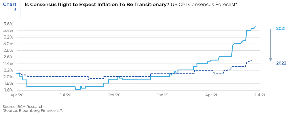
Airfare, hotel rates, and event tickets are also rising as the general population remerges from pandemic lockdowns. Consumer spending has further been inflated by temporary transfer payments disbursed through various pandemic-fighting fiscal programs which are set to expire in September. This portends a 2022-23 reversal of the positive fiscal thrust of 2020-21 (Chart 2). The Biden Administration’s pared down infrastructure bill is unlikely to be immediately disbursed through big “shovel ready” projects ready to go from day-one and thus, would not be expected to impact the economy immediately. The American Jobs Plan would inject another $1 trillion or so, and the European Union’s Next Generation Plan does the same, so both plans together could be structurally inflationary. However, and particularly in the U.S., this additional fiscal largesse will need to be financed by a variety of tax increases: corporate, personal, and capital gains. This will greatly reduce the net fiscal stimulus.
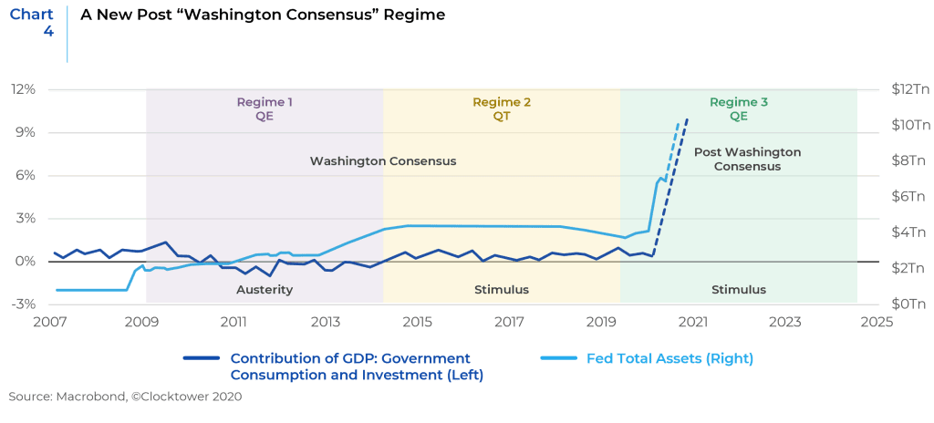
Consequently, market expectations, as measured by the 10-year TIPS breakeven inflation expectations (which is hovering around 2.3%), as well as expectations that the first Fed rate hike taking place by the end of 2022, are consistent with the belief that current spikes in inflation are transitory. (Chart 3).
But there is a risk to the “transitory” consensus; more specifically, how long will a “transitory” period last?
Historically, persistent inflationary episodes have been associated with three factors, individually or jointly: (i) sustained demand in excess of supply; (ii) sustained wage increases in excess of labor productivity growth, reflecting changes in the bargaining power of workers and employers; and (iii) de-anchoring of inflation expectations.
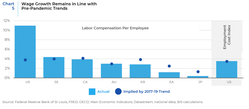
The first factor (the balance between aggregate demand and supply) is determined primarily by the effectiveness and timeliness of monetary and fiscal policy interventions. G7 central bankers have understandably erred thus far on the side of being too easy after decades of fighting disinflationary pressures by keeping rates extremely low. The difference from recoveries during the last three recessions is the relative health of private sector balance sheets and the magnitude of the fiscal policy response. For example, the 2009 American Recovery and Reinvestment Act sparked the tea party political revolution, which putatively stood for fiscal prudence and austerity. Consequently, from 2010 to 2016, the US had a long period of self-imposed austerity, whereby government was not contributing to GDP growth. The question today is whether the policy response to COVID is indicative of a one-time response to a crisis, or representative of the dawn of a new framework of thinking about economic policy. More specifically, could we be shifting away from the 40-year-old “Washington Consensus” characterized by fiscal austerity, privatization, globalization, supply side and the almost unfettered laissez faire economics of Reagan and Thatcher to a new orthodoxy? (Chart 4).
Despite yawning differences on so called social “wedge” issues, polls on median voter preferences suggest less tolerance for free trade and austerity and greater demands for keeping entitlement spending at current and largely unsustainable levels.1 The subtle changes in the Fed’s announced focus on full employment and employment/income disparity may be consistent with a post-Washington economic paradigm, which could lead to an era of higher and less stable inflation.
With respect to wage increases, despite an all-time high in job openings (as measured by JOLTS), important measures such as the Atlanta Fed Wage Tracker suggest that higher consumer prices are not (yet) feeding through into higher wages. Globally, labor compensation per employee – a broad measure of wages – remains in line with its pre-pandemic trend in most economies, and is somewhat below trend in Korea, the Euro area and Japan. (Chart 5). With labor compensation per employee more than 6 percentage points above its pre-pandemic trend, the U.S. is the sole exception. But the U.S. trend is distorted by a pandemic-induced change in the labor force composition. Job losses were concentrated among low-income workers, which arithmetically increased the level for the remaining workers. The U.S. Employment Cost Index (shown on the right of Chart 5) controls for changes in the labor force composition. Thus far, this index shows little indication of accelerating wage growth.
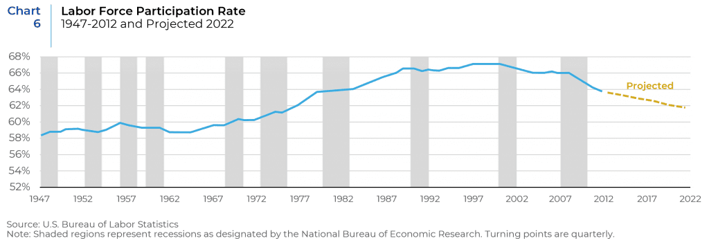
It is important to remember that the drivers that anchored wage inflation in the 1960s and 1970s are very different today. Unionized workers in the 1970s were 25% of the labor force; today, they only represent around 10%. Labor unions introduce wage rigidity, a key reason behind that period’s wage-price spiral. Today, most workers in the U.S. compete for jobs both at home and abroad, which is further compounded by low-wage countries as a result of globalization. Also, as the “Fourth Industrial Revolution” advances, rapid digitization, robotic technology, AI and 5G communication are inherently deflationary. This goes a long way towards explaining why the Fed has not been able to “push” inflation up to its target for more than a decade. But there are also secular trends that could be supportive of a higher and less stable inflation environment. The ongoing politicization of trade globalization could, at the margin, reduce an important deflationary impulse in wage costs. Additionally, even accounting for the employment shortfall related to workers sidelined by generous unemployment benefits and/or health or childcare related concerns, demographic factors such as retiring baby boomers, fewer youths and prime “working age” individuals are leading to a structural decline in the labor force participation rate. (Chart 6). This rebalancing, as well as the political/policy changes discussed above, could provide support for higher overall wages.
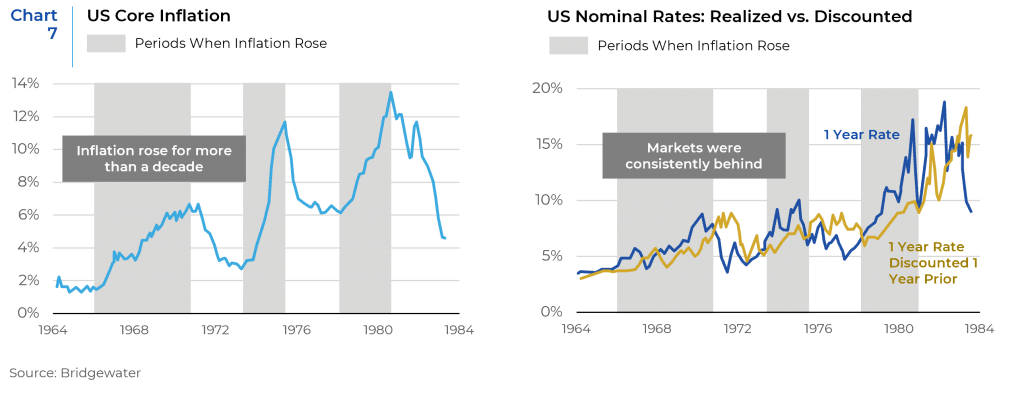
The third factor, a de-anchoring of inflation expectations, is the hardest to predict and the most pernicious. All macroeconomic regimes are undergirded by a psychological element or zeitgeist. For example, infrastructure spending could further pressure the labor market even after workers return to the labor force when pandemic-related benefits expire in September. A psychological inflationary feedback loop could be catalyzed by continued tightness in the labor market, and/or robust consumption (as consumers spend down the savings they have squirreled away during the pandemic), which would accommodate higher prices. If supply-side constraints continue, high commodity prices could also trigger a feedback loop. This is why market consensus for interest rate movements historically lagged actual experience during high and rising inflation periods in the 1960s and 1970s. (Chart 7). This pattern suggests an intermediate term risk that both the market consensus and the Fed are too complacent and that the FOMC will need to hike rates sooner and higher than currently discounted.
Implications for Investors/Asset Allocators
For investors/allocators, a sustained upward inflation surge or greater inflation volatility could materially challenge current equity valuations and upend the fundamental premise underpinning investors’ asset allocation models – that stocks and bonds are likely to be negatively correlated and naturally diversifying.
Because rising inflation diminishes the present value of cash flows generated by bond yields, fixed income returns are typically challenged in high inflation environments. For this reason, low or falling inflation environments (i.e., the last 30+ years) flattered the bond market. For equities, company sales are typically supported by rising nominal growth; but higher inflation can also increase costs, which would hurt margins. Moreover, for both stocks and bonds, rising interest rates would put upward pressure on the discount rate used to value assets. This is particularly challenging in today’s environment of negative real interest rates across the developed world and relatively high U.S. equity valuations (at least based on cyclically adjusted valuations). Low nominal yields and negative real yields on bonds mean much of investors’ portfolios are now providing unacceptably low returns and more limited diversification. High equity valuations likewise reduce expected future returns, and so a market-cap-weighting approach increases this vulnerability by causing investors to hold more of the same assets that are now yielding less.
Below, we update our 2019 analysis on the changing relations in periods of high inflation and stagflation. Because of the small sample size available for historical stagflation periods, we extended the analysis using inflation expectations to define both inflationary and stagflationary periods between 1970 and Q2 2021 (Table 1). Our approach is consistent with prior research that demonstrated that inflation surprises are a more significant driver of asset returns than just the level of inflation.2 We defined inflation surprises as the difference between actual inflation at the end of the quarter and expectations for inflation at the start of the quarter with a period being designated as “high inflation” if the surprise is in the highest 25% of historical experience. Additionally, we measured stagflationary periods as times during which GDP growth was in its bottom 25% and inflation was in its top 25%.
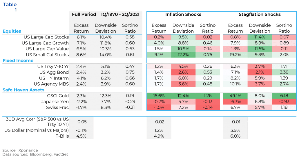
The table evaluates excess U.S. large cap equity returns relative to 3-month T-Bills; 6.1% over the full period, 0.2% during inflation “surprise shock” periods, and 0.8% for stagflation periods. For bonds (as measured by the U.S. Treasury Bond Index), the full period excess return was 2.4%, 1.2% during inflationary periods and 6.3% during stagflationary periods. The table also evaluates the Sortino ratio for each asset; which is a modified version of the Sharpe Ratio (by penalizing downside volatility). Due to smaller drawdowns, bonds outperformed stocks on a risk-adjusted basis during both periods (excepting small cap stocks which outperformed). Among bond sectors, Core bonds (as represented by the U.S. Agg bond index) had a higher Sortino ratio than other sectors and US Agency MBS had the second highest ratio in both periods; suggesting that sector diversification within fixed income portfolios could partially offset a deleterious inflation effect. Not surprisingly, gold also outperformed in both periods, which underscores the value of incorporating hard or real assets in a portfolio to hedge against inflation.
Chart 8, which evaluates the correlation between stocks and bonds relative to inflation, demonstrates that the diversification benefit of owning stocks and bonds is disproportionately high in low inflation regimes. Since bond prices have an inverse relationship with yields, a positive correlation between S&P returns and yields suggests a negative relationship between equity and bond returns.
Finally, Chart 9 provides a longitudinal analysis of stock/bond correlations and the inflation relationship.
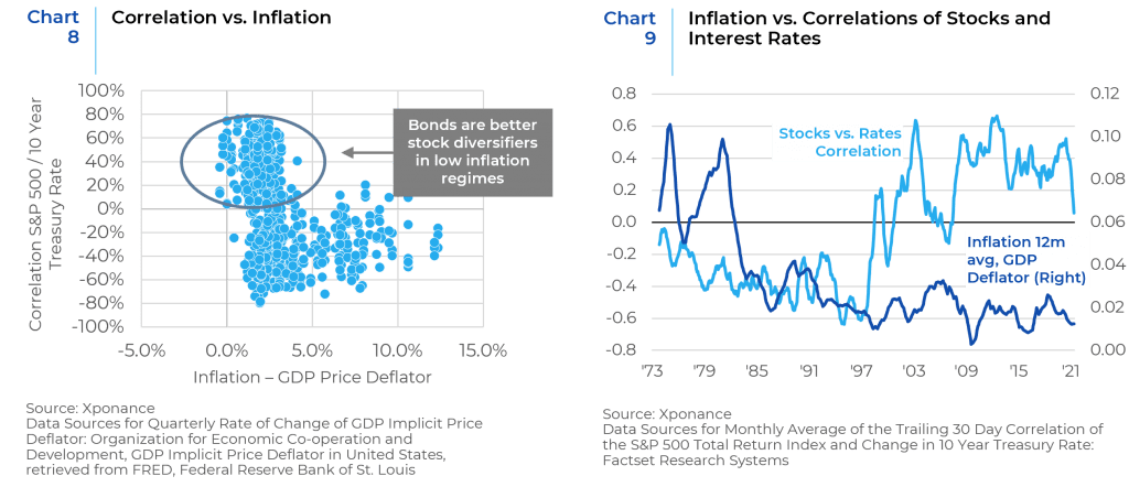
During high inflation periods of the 1970s and early 1980s, stocks and interest rates were negatively correlated, which means that stock returns and bond returns were positively correlated. In the early 1980’s, Fed Chair Paul Volcker’s “cold bath” strategy to tame inflation (by hiking rates to as high as 20%) caused a regime shift which thereafter was characterized by falling and/or stable inflation. In this environment, the primary drivers of asset prices were growth, and a readjustment of the risk premium associated with major changes in market liquidity. Inflation became a far less important driver. Consequently, stock prices and bond yields became positively correlated while government bond prices/returns, and stock prices were negatively correlated. This dynamic enabled investors to easily diversify their equity holdings through bond allocations.
Going forward, we do not believe that current price pressures are the “real story” for investors making long term asset allocation decisions. While we are sympathetic to the view that most of the recent price increases are likely transitory, one must also acknowledge that prolonged “transitory” inflation can lead to a de-anchoring of inflation expectations, particularly if the Fed gets too far behind the curve However, for investors making long term asset allocation decisions, the secular risks of less stable and higher inflation are meaningful, and asset allocation models that simply evaluate relationships over the last three decades could be vulnerable to such a regime shift. Accordingly, investors should consider hedging against a higher and more volatile inflation regime by increasing their allocation to hard/real assets.
1 See for example, the Spring 2014 Global Attitudes Survey by Pew Research
2 See for example, Page, Pedersen and Guo (PIMCO), Inflation Regime Shifts Implications for Asset Allocation. October, 2012
This report is neither an offer to sell nor a solicitation to invest in any product offered by Xponance® and should not be considered as investment advice. This report was prepared for clients and prospective clients of Xponance® and is intended to be used solely by such clients and prospects for educational and illustrative purposes. The information contained herein is proprietary to Xponance® and may not be duplicated or used for any purpose other than the educational purpose for which it has been provided. Any unauthorized use, duplication or disclosure of this report is strictly prohibited.
This report is based on information believed to be correct, but is subject to revision. Although the information provided herein has been obtained from sources which Xponance® believes to be reliable, Xponance® does not guarantee its accuracy, and such information may be incomplete or condensed. Additional information is available from Xponance® upon request. All performance and other projections are historical and do not guarantee future performance. No assurance can be given that any particular investment objective or strategy will be achieved at a given time and actual investment results may vary over any given time.