
Part 3: Evaluating Rebalancing Techniques for Portfolio Derisking
In this, the third of a three-part series “Battening Down the Hatches”, we evaluate portfolio derisking techniques that most cost effectively allow allocators to re-attain their pre-recession asset levels and funding levels. To recap, in Part 1 of this series, we reviewed the case for portfolio derisking. In Part 2, we evaluated the macro background, asset return sensitivities, and market responses during economic downturns over the last 30 years; the stagflation periods of the 1970s and 1980s as well as periods of heightened changes in inflation expectations and bottom quartile growth from 1970 to the present. However, because several key variables, (such as bond yields, inflation, valuations, monetary policy settings and growth) are very different today than at the beginning of these past downturns, we discussed asset protection or return expectations and assumptions that need to be revisited.
In this installment, we determine how effective three classic portfolio derisking techniques would have been in restoring plans to their pre-recession asset and funding levels.
The three approaches analyzed are:
- Annual rebalancing that maintains pre-recession asset weights.
- A dynamic derisking model which uses observable market and economic signals to reduce and increase a portfolio’s equity risk.
- Using equity index options to hedge downside risk.
Our model is based on the asset allocation and financial profiles of the 103 state plans that were included in Wilshire Associates’ 2019 report on State Pension Plans. We evaluate each technique’s performance over three prior recession periods: the 1990 recession; the Dot Com crash and the GFC (please see the inset below for a recap on each of these periods).
Our analysis showed that an annual rebalancing strategy to maintain pre-recession asset allocation weights would have re-attained most state plans’ prior funding ratios for all but the Great Recession. Our dynamic derisking model appeared to be most effective during severe recessions but in all cases would be expected to reduce a plan’s maximum drawdown as well as the decline in their funding ratios relative to the more passive annual rebalancing approach. However, dynamic models are heavily dependent on timing, as most economic and market indicators tend to operate with a significant lead time and are prone to false positives. Unfortunately, in the real-world, unknown timing would force an allocator to “wait out” false positives, compounding their mistake. With low to negative bond yields, the opportunity cost of derisking prematurely is higher than ever because liabilities would grow faster than one can earn on safe assets. This is why we believe that allocators should also consider index options strategies to hedge equity downside risks. In effect, a derisking strategy using options would allow allocators to size their option position to achieve a target downside risk without giving up the upside potential of equities for low yielding bonds. This is not to imply that derisking through options is without cost. In the case of false positives, the allocator would bear the cost of purchasing the option at its expiration, without an offsetting gain from the trade. However, we found that relative to rebalancing physical assets to a conservative portfolio, using just 1% to 2% of a portfolio’s equity assets to purchase deep out of the money put options would be expected to generate higher returns; even when factoring in hedging costs.
Chart 1, Table 1 and Table 2 characterize key characteristics of the state plans from the aforementioned Wilshire study.
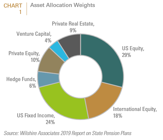
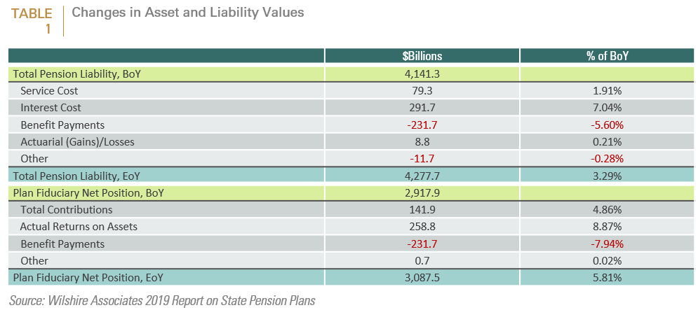
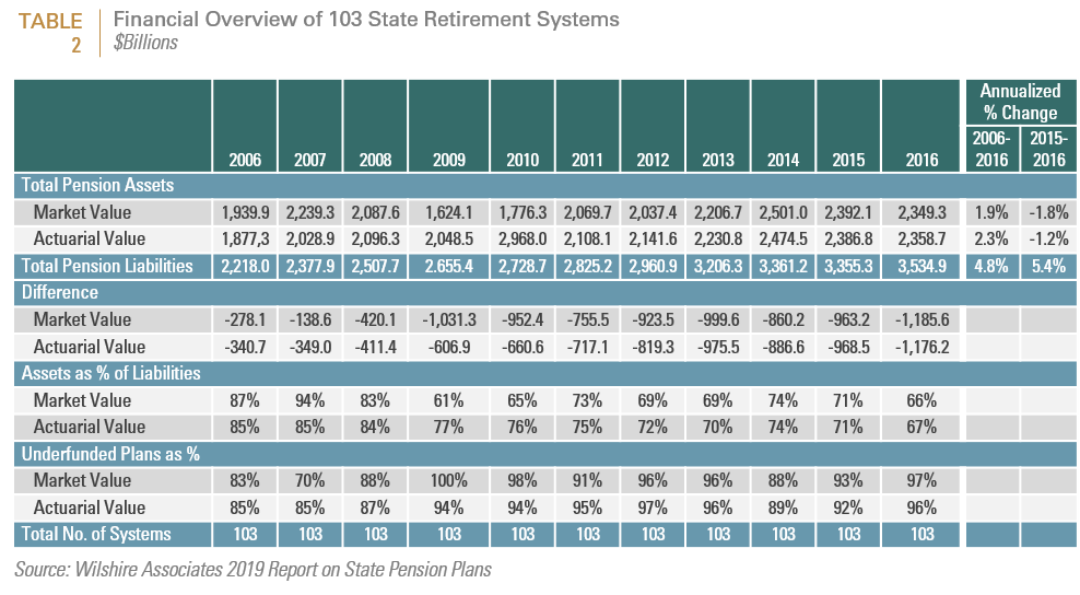
Chart 1 depicts the asset allocation weights used in our model. Based on the contributions and benefits payments data compiled in the state pension plan study (Table 1), we assume a 3.4% growth in pension liabilities as well as a negative outflow of 3.1% to fund benefits and plan operations. This estimate of liability growth is lower than actual growth for the decade ending in 2016 (see TABLE 2). This means that in order to maintain funding levels, state pension plans as a group would need to grow their assets between 7% to 8%.
With this profile as a backdrop, we evaluate the effectiveness of the three aforementioned derisking techniques in restoring plans to their pre-recession asset and funding levels.
Derisking Through Annual Rebalancing
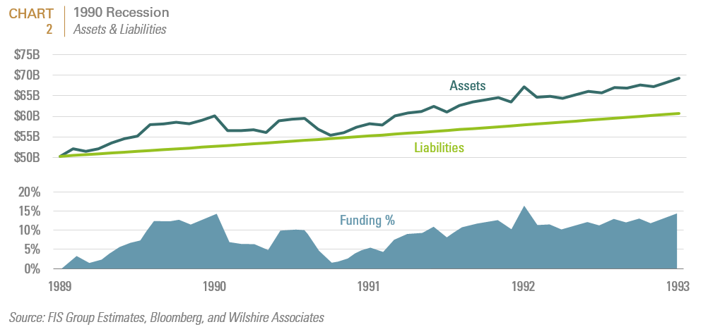
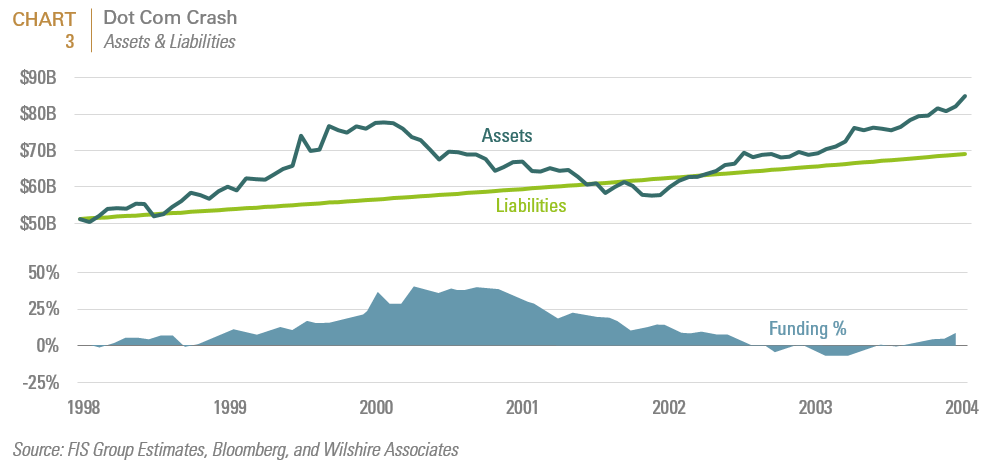
The annual rebalancing method straightforwardly restores initial asset allocation weights at the end of each calendar year, when possible, through liquid asset classes. For Private Equity and Venture Capital, we assume that additions can be made annually, but cuts were only made every 5 years. Our analysis suggests that for both the 1990 and Dot Com recessions, asset levels and funding ratios fell significantly but quickly recovered above baseline levels after the recovery (see Chart 2 and Chart 3).
Recapitulation of the Three Recession Scenarios
Table 3 recaps salient characteristics of the three recessions that were evaluated in our model.
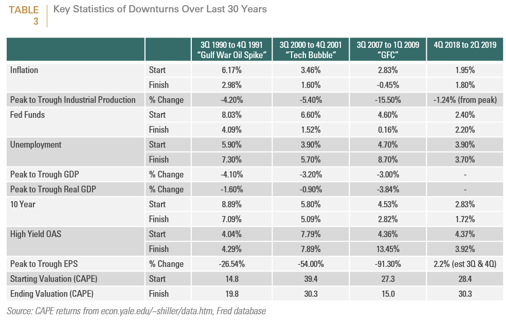
All three downturns were preceded by rising interest rates as a result of Fed policy. The 1990’s “tight money” recession was the mildest of the three and could also be considered as a mild supply shock recession in that it was also precipitated by the invasion by Iraq into Kuwait. This resulted in a spike in the price of oil in 1990, which caused manufacturing trade sales to decline. The stock market decline of -6.56% in 1990 was also precipitated by the collapse of the leveraged buyout of United Airlines in 1989. For both the Tech bubble and the GFC, industrial production respectively declined by 5.4% and 15.40%. Notably, both were caused by the bursting of an asset bubble in which valuations became detached from their intrinsic value in the case of Dot Com and telecom stocks, and unsustainable relative to income levels in the case of the housing bubble.
The table suggests three key differences between today’s macro backdrop and the prior periods. First, as of June 30, 2019, the equity markets’ cyclically adjusted (CAPE) valuation of 30.3 is higher than it was at the end of all bull markets that preceded a subsequent equity and cyclical downturn with the exception of the end of the Dot Com era. The other glaring differences are levels of inflation, the yield on 10-year treasuries and the fed funds rate. As of June 30, 2019, the fed funds rate stood at 2.2% vs. 8.03% at the beginning of the 1990 downturn; 6.60% at the beginning of the dot com downturn and 4.06% at the beginning of the GFC. Given that allocator’s liabilities are either directly discounted by or related to the yield on 10-year treasuries, today’s low yield levels would increase the opportunity cost of premature derisking.
For the GFC however, whereas the plans’ asset levels have recovered, as of June 30, 2019, funding levels for the most part have not reached their pre-2008 levels. Specifically, between 10/2007 and 6/2019, the state funds’ asset allocation would have returned approximately 5%; while as indicated previously, roughly 7% to 8% is needed to keep pace with liability growth (3.4-4.8% growth in liabilities plus ~ 3% in cash flow needed to fund current outflows (see Chart 4).
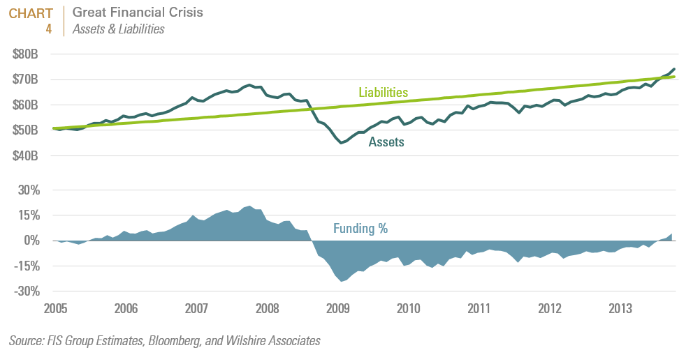
The temptation to ‘time’ the market likely stems from the fact that post crisis returns (3/2009 – 6/2019) have been very strong 10.5%; but not enough to dig out of the 30% loss during the drawdown (11/2007-2/2009). In order to address this shortfall, plans have been increasingly shifting into illiquid assets with higher return assumptions; but even that has been insufficient to achieve 8% annualized returns, given the low interest rate environment (which lowers returns from bonds and cash).
We turn next to analyzing a more dynamic model which shifts the allocation from riskier (equity) assets to safety assets (bonds), based on observable market-based and economic signals.
Dynamic Derisking
Our dynamic model uses two observable signals. The first is the inversion of the yield curve (as measured by the difference between the 2-year and 10-year bonds) and the second is the New York Federal Reserve’s recession probability indicator. While neither indicator is perfect and can lead to either false positives and varying lags, both are widely watched measures of future economic declines.
Using these two indicators, our dynamic derisking model rules were as follows:
- Start the derisking process the quarter after a yield curve inversion (10-2yr).
- The derisked portfolio would cut the equity weight by 50% and reallocate the proceeds as follows:
- 50% to US fixed income
- 25% to hedge funds
- 25% to private equity
- Maintain derisked portfolio positioning until 2 quarters after recession probability falls below 10%
These model rules led to the following signals:
| 12/31/1988 | Derisk |
| 3/31/1992 | Rerisk |
| 6/30/1998 | Derisk |
| 9/30/2002 | Rerisk |
| 3/31/2006 | Derisk |
| 3/31/2010 | Rerisk |
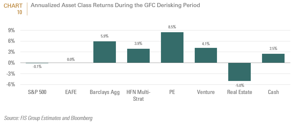
Using the previously referenced recession scenarios, the results of this model relative to the primary goals of restoring a plan’s assets and funding ratio are demonstrated in Chart 5 through chart 10.
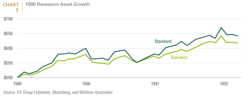
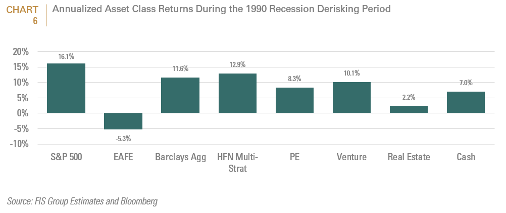
For the relatively mild 1990 recession, the dynamic derisking strategy would have underperformed the more passive annual rebalancing approach; mostly because it would have kept plans at too low an equity exposure for too long. As shown, equities actually outperformed during the full derisking period (see Chart 6).
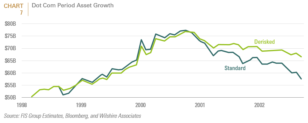
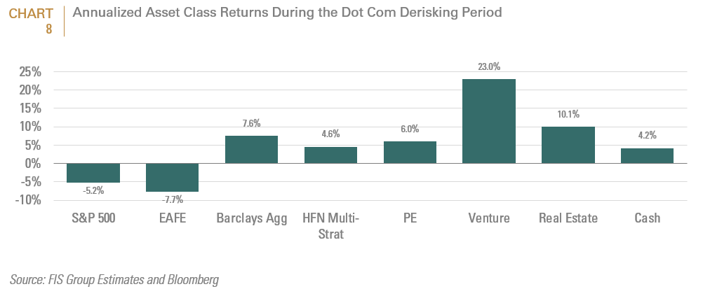
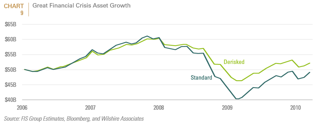
On the other hand, the dynamic derisking strategy would have outperformed during the much more severe Dot Com (Chart 7 and Chart 8) and GFC (Chart 9 and Chart 10) recessions.
However, following this strategy would have required steadfast discipline. For example, 18 months into the decision to derisk during the Dot Com recession would have set the plan back by 3.8% of assets (the S&P 500 index returned 32.2% from 6/98-12/99 while the Barclays Aggregate Index returned 3.7%). The decision to derisk would have paid off, but only after a year and a half of sharp underperformance.
Dynamic derisking would also have helped during the GFC because of the strong performance generated by core bonds, hedge funds and private equity; all of which, to varying degrees would have received increased exposures from our model (see Chart 10).
Table 4 summarizes the key results for the dynamic model for each of the recession scenarios. The dollar amounts model a fully funded state plan with $50 billion under management with the start date and end dates listed in the table. The dates were extended past the charts to capture the months to recovery when possible.
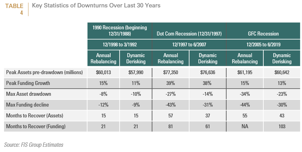
The table confirms that in all cases, the dynamic model would have been expected to reduce a plan’s maximum drawdown as well as the decline in their funding ratios. As would be expected, the recovery time with respect to both assets and funding ratio varied with the severity of the recession; with the GFC being the most severe and the 1990 recession being the mildest of the three scenarios. Moreover, as discussed above, the benefits of the dynamic strategy increased with the severity of the recession. For example, for the mild 1990 recession, dynamic derisking would not have been particularly fruitful. However, for the Dot Com crash, dynamic derisking would have cut a plan’s maximum drawdown by almost 50%. While the plan would have recovered in terms of peak assets in 57 months through an annual rebalancing strategy, the recovery time would have been cut to 37 months through dynamic derisking. Importantly, while this plan (assuming the cash flow and liability growth rates previously referenced) would have taken 81 months to recover pre-recession funded ratios, with dynamic derisking, the plan’s pre-recession funded ratio would be restored in 61 months. For the GFC, dynamic derisking would have cut a plan’s maximum drawdown by approximately 28%. While the plan would have recovered in terms of peak assets in 55 months through an annual rebalancing strategy, the recovery time would have been cut to 43 months through dynamic rebalancing. While annual rebalancing would still not restore pre-recession funded ratios as of the end date, with dynamic derisking, the plan’s pre-recession funded ratio would be restored after 103 months.
This analysis suggests that dynamic derisking appears to be more protective of an allocator’s pre-recession assets and funded ratios, particularly for more severe recessions. However, it is important to note that the derisking scenarios we have laid out have the benefit of hindsight. Specifically, our models have the unrealistic luxury of knowing that the yield curve inversion was forecasting a recession. Setting up a rule to ‘derisk’ and wait is easy to do, when one knows the recession and market correction will come. The primary issue is that the indicators chosen (yield curve inversions and the New York fed recession probability index or any macro model) must balance being sensitive enough to capture all recessions without increasing the number of false positive signals generated.
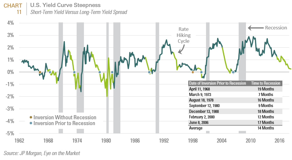
Both of these heavily watched indicators and, indeed most such indicators have a history of being too sensitive, with false positives and long lead times. The yield curve, for example, has predicted every recession in the past 50 years. However, it also predicted 2 recessions that never occurred and the lag between inversion and the subsequent recession has varied between 2 months and 18 months (see Chart 11 as well as Part 1 of this research series for a fuller discussion on the yield curves’ efficacy as a recession indicator).
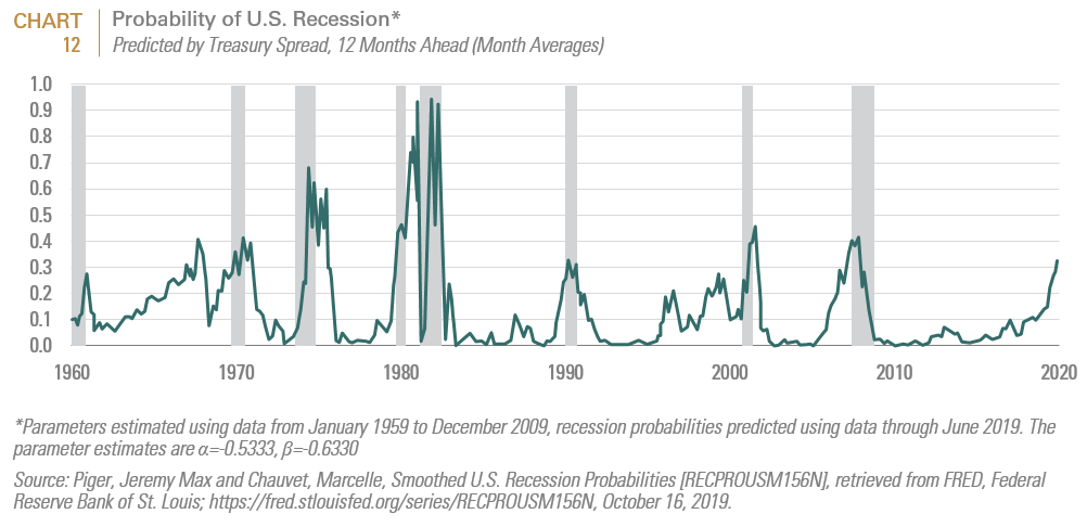
The New York Federal Reserve’s probability model, which predicts the probability of a U.S. recession in the next 12 months, has breached the 30% threshold before every recession since 1960. To calculate recession probability, the New York Fed’s tracker gauges the difference between the 10-year and 3-month Treasury rates. However, like the yield curve, this indicator has also suffered from highly variable lags between the signal and the subsequent recession (see Chart 12).
Unfortunately, in the real world, unknown timing would force an allocator to “wait out” false positives, compounding their mistake. With low to negative bond yields, the opportunity cost of derisking prematurely is higher than ever because liabilities would grow faster than one can earn on safe assets. One way of addressing this opportunity cost is to use an options strategy to truncate the portfolio’s downside from an equity drawdown.
Derisking through index options strategies
Chart 13 shows the total cumulative return for a “full” risk standard portfolio (67% S&P500 stock index and 33% Barclays Aggregate bond index) vs. a more conservative portfolio (33% S&P 500 stock index and 67% Barclays Aggregate bond index) for the 5 quarters after yield curve inversions since 1972. In order to directly compare these options with an options strategy, we chose 5 quarters due to the liquidity of options available at year end expirations. Additionally, rather than using historical returns of bonds, we chose current rates to estimate fixed income returns (2.88% total return over 5 quarters).
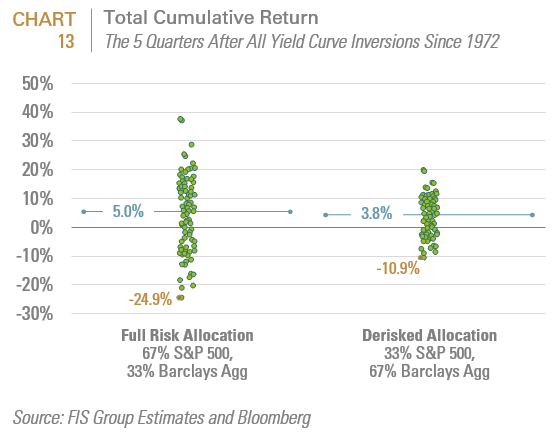
While the conservative portfolio truncated the portfolio’s maximum downside, it also truncated its upside and more importantly, led to a lower average return level than the full risk portfolio. Moreover, physically rebalancing assets into the more conservative portfolio could be expensive and technically incur unlimited funding risk, because there is no limit as to how far the equity portfolio which was sold, could rise in price after the investor sold its shares. Fortunately, options could offer less costly alternatives.
A put or put option gives the owner the right to sell an asset (in this case, the S&P 500 index), at a specified price, by a predetermined date to a given party. A put option is out of the money (OTM) if the underlying index’s price is above the strike price. If at expiration, the S&P 500 index remains above the strike price, the option expires worthless and ceases to exist, leaving the investor with the cost of purchasing the option. We chose an OTM put to reduce the potential investor’s hedging costs.
If an allocator purchased roughly 10% OTM put option on the S&P 500 index expiring mid-December 2020 with 4.3% of their portfolio, the maximum loss on their stock portfolio we be around 14% (10% drawdown + cost of options). (See the panel below).
SPDR S&P 500 ETF Trust Put DEC20 270.00 (LEAPs)
Below is the same analysis as the prior chart with 1% increments taken from an investor’s equity portfolio and used to purchase a hypothetical OTM put option with the same pricing and characteristics referenced, held to expiration. Not surprisingly, the level of downside protection increases with increasing increments of put protection. But this downside protection is not without costs, because in the case of false positives, an allocator would bear the cost of purchasing the option at the option’s expiration without an offsetting gain from the trade. However, relative to reallocating their portfolio’s physical assets to the conservative portfolio shown in Chart 13, both the 1% and 2% hedge options generated higher average returns; even when factoring in hedging costs (see Chart 14).
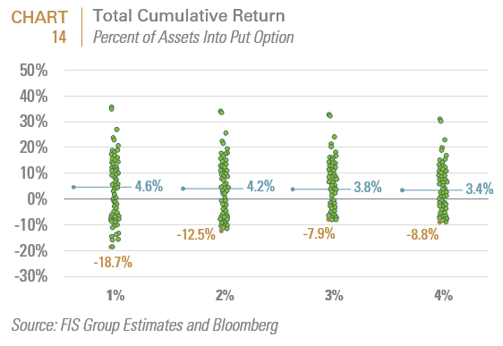
In effect, a derisking strategy using options would allow allocators to size their option position to achieve a target downside risk without giving up the upside potential of equities for low yielding bonds.
The above options analysis illustrates a basic downside protection approach using put options. Allocators should consider more sophisticated strategies that could either reduce their hedging expense or increase their expected risk-adjusted return. Here are some options worth exploring:
- Currently, it is cheaper to hedge developed international stocks with a January 2021, 10% OTM put on developed non-U.S. equities (as represented by the EAFE index) costing only 3.37% (compared to 4.3% for the S&P 500 index). Using this instrument would reduce hedging costs.
- Currently, OTM puts on the Russell 1000 Growth cost less than the S&P 500 index OTM put (4% vs 4.3%). Given the risks facing growth stocks, and historically high valuations, this provides another interesting opportunity to reduce hedging costs.
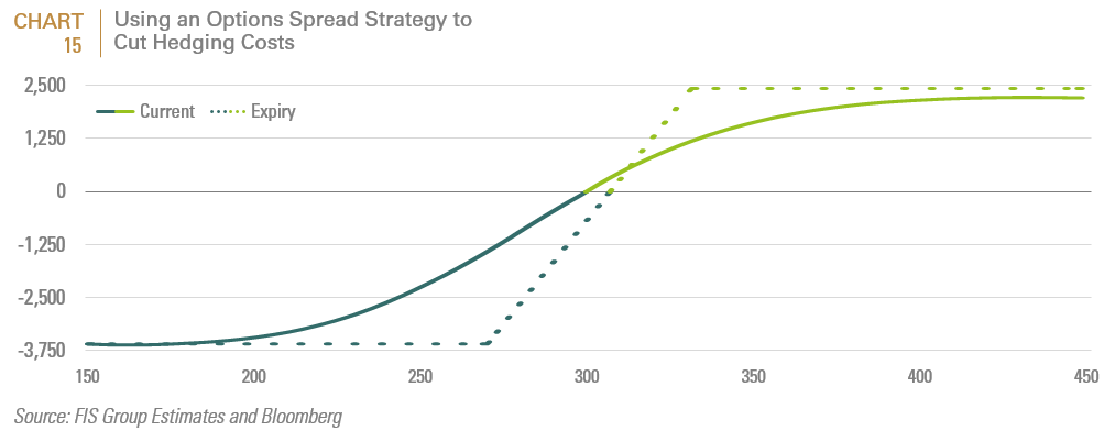
- Options spread strategies. For example, selling a 10% OTM call option on the S&P 500 index in addition to purchasing the put previously discussed, would cut an investor’s hedging cost in half. The cost however would be that the upside return on their stock portfolio would be limited to 8% (see Chart 15).
Summary
Table 5 summarizes our findings. The table ranks each strategy relative to both the severity of the recession and the duration of the funding requirement.
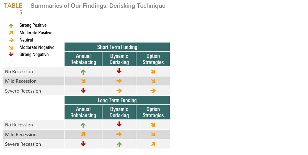
So for example, annual rebalancing works best for no recession and worst during severe recessions.
Our dynamic derisking model was most effective during severe recessions but in all cases would be expected to reduce a plan’s maximum drawdown, as well as the decline in their funding ratios relative to the more passive annual rebalancing approach. However, dynamic models are heavily dependent on timing; as most economic and market indicators tend to operate with a significant lead time and are prone to false positives. Moreover, as discussed in Part 2 of the research series, in light of historically low starting yields on core fixed income securities, (the most common destination for derisking strategies), the opportunity cost of ill-timed derisking could be significant because an allocator would be forced to “wait out” false positives, while their liabilities grow much faster than safety assets. This is why we believe that allocators should also consider index options strategies to hedge equity downside risks. In order to reduce the hedging costs associated with purchasing downside protection, we recommended OTM put options as well as other strategies designed to reduce the cost of hedging. This is why we have rated this strategy as “moderate negative” for no or mild recessions; because a mild recession and its associated market decline would be less likely to trigger the option’s strike price, leaving it to expire worthless.
Important Disclosures:
This report is neither an offer to sell nor a solicitation to invest in any product offered by FIS Group, Inc. and should not be considered as investment advice. This report was prepared for clients and prospective clients of FIS Group and is intended to be used solely by such clients and prospects for educational and illustrative purposes. The information contained herein is proprietary to FIS Group and may not be duplicated or used for any purpose other than the educational purpose for which it has been provided. Any unauthorized use, duplication or disclosure of this report is strictly prohibited.
This report is based on information believed to be correct, but is subject to revision. Although the information provided herein has been obtained from sources which FIS Group believes to be reliable, FIS Group does not guarantee its accuracy, and such information may be incomplete or condensed. Additional information is available from FIS Group upon request.
All performance and other projections are historical and do not guarantee future performance. No assurance can be given that any particular investment objective or strategy will be achieved at a given time and actual investment results may vary over any given time.